Cassin’s vireo

This notebook walks through a complete chatter workflow using recordings of Cassin’s vireo as a worked example. It is intended to be the main, end-to-end tutorial for the Python package, showing how each component fits together.

We will:

• Configure chatter for this dataset (sampling, frequency range, segmentation options).

• Preprocess raw audio and extract clips that contain Cassin’s vireo songs and calls.

• Segment clips into individual acoustic units and save standardized spectrograms.

• Train a convolutional variational autoencoder (VAE) on those spectrograms.

• Extract features from the trained model.

• Post-process and visualize the learned latent space and a set of derived acoustic measures.

If you are new to chatter, please read this notebook in its entirety and use it as a template for your own species or datasets.

The Cassin’s vireo recordings come from:

Hedley, R. W. (2016). Complexity, predictability, and time homogeneity of syntax in the songs of Cassin’s vireo (Vireo cassinii). PLOS ONE. https://www.doi.org/10.1371/journal.pone.0150822

© Michael Stubblefield (eBird S108126823)

Setup

In this section we import chatter and a few standard scientific Python libraries, then define a configuration that controls every major step of the pipeline.

Key ideas:

• Configuration dictionary: we start with a Python dict containing only the parameters we want to override (e.g., frequency range, preprocessing filters, segmentation thresholds). chatter.make_config fills in all remaining fields with sensible defaults.

• Analyzer: chatter.Analyzer orchestrates preprocessing, segmentation, and spectrogram creation. It is initialized with a config and the number of CPU cores to use (n_jobs).

• Trainer: chatter.Trainer wraps the autoencoder model and training loop.

• Paths: we keep all file system paths in clearly named variables (raw_dir, input_dir, processed_dir, h5_path, csv_path, model_dir, output_csv_path) so you can easily adapt this notebook to your own directory structure.

When adapting this example, you will typically:

1. Adjust the config values to fit your species or recording conditions.

2. Change the path variables to point to your own data locations.

3. Optionally change n_jobs based on how many CPU cores and how much RAM you have available.

First we import Chatter and a few core scientific Python libraries. These imports are all you need to follow along with this notebook and run the full pipeline on your own data.

# import packages
import chatter
from pathlib import Path

This next cell defines our analysis configuration and initializes the main Chatter objects. We override a few defaults (e.g., frequency range and segmentation settings), call make_config() to fill in the rest, construct an Analyzer and Trainer, and then specify all the key paths on disk for this example dataset.

# set config parameters that depart from defaults
config = {
    # spectrogram parameters
    "fmin": 1500,
    "fmax": 7500,
    # preprocessing parameters
    "use_biodenoising": True,
    "use_noisereduce": True,
    "high_pass": 1500,
    "low_pass": 7500,
    "static": True,
    "threshold": 2,
    # simple segmentation parameters
    "simple_noise_floor": -60,
    "simple_silence_threshold_db": -50,
    "simple_min_silence_length": 0.01,
    "simple_max_unit_length": 0.8,
    "simple_min_unit_length": 0.1,
    # other parameters
    "plot_clip_duration": 5,
}
config = chatter.make_config(config)

# initialize the analyzer with the configuration
# using only 8 cores to avoid memory crash during segmentation
analyzer = chatter.Analyzer(config, n_jobs=8)
model = chatter.Trainer(config)

# set paths
raw_dir = Path("/Volumes/Expansion/data/chatter/examples/cassins_vireo/recordings/raw")
input_dir = Path(
    "/Volumes/Expansion/data/chatter/examples/cassins_vireo/recordings/clips"
)
processed_dir = Path(
    "/Volumes/Expansion/data/chatter/examples/cassins_vireo/recordings/processed"
)
h5_path = Path("/Volumes/Expansion/data/chatter/examples/cassins_vireo/spectrograms.h5")
csv_path = Path(
    "/Volumes/Expansion/data/chatter/examples/cassins_vireo/spectrograms.csv"
)
model_dir = Path("/Volumes/Expansion/data/chatter/examples/cassins_vireo/model")
output_csv_path = Path(
    "/Volumes/Expansion/data/chatter/examples/cassins_vireo/output.csv"
)
output_html_path = Path(
    "/Volumes/Expansion/data/chatter/examples/cassins_vireo/cassins_vireo_embedding.html"
)

Using 8 cores for parallel processing
Initializing convolutional variational autoencoder
Using device: mps

Preprocessing

Raw field recordings are typically long, noisy, and contain many species. In chatter we break the problem into two or three stages before segmentation:

1. Species-specific clip extraction (extract_species_clips) (optional):

   • We scan the raw directory with BirdNET and keep only the time intervals where Cassin’s Vireo is detected above a chosen confidence threshold.

   • Each detection is exported as a short WAV file into input_dir, preserving a directory structure that mirrors the original recordings.

2. Preprocessing demo (demo_preprocessing):

   • Before batch-processing everything, we take one random clip and run it through the full preprocessing pipeline in memory.

   • This produces a diagnostic plot so you can visually confirm that filters, denoising, and normalization look reasonable for your data.

3. Batch preprocessing (preprocess_directory):

   • We then apply the same preprocessing operations to every clip in input_dir and save standardized WAV files (same sample rate, channels, and loudness) into processed_dir.

For your own data, you can skip step 1 if you already have species-specific clips, but it is often useful when starting from long, mixed-species recordings.

We start by extracting clips that actually contain Cassin’s vireo. extract_species_clips() scans long raw recordings in raw_dir with BirdNET, identifies segments where the target species is present above the specified confidence threshold, and writes those segments as shorter WAV files into input_dir.

# identify and export clips with cassin's vireo
analyzer.extract_species_clips(
    input_dir=raw_dir,
    output_dir=input_dir,
    species="Cassin's Vireo",
    confidence_threshold=0.99,
)

--- Found 221 audio files to process ---

Detecting 'Cassin's Vireo': 100%|██████████| 221/221 [09:51<00:00,  2.67s/it]

--- Species clip extraction complete. Clips saved to /Volumes/Expansion/data/chatter/examples/cassins_vireo/recordings/clips ---

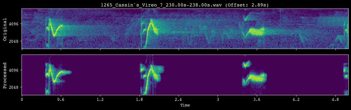
Before launching full preprocessing, we run a quick visual check. demo_preprocessing() selects a single clip, applies the same preprocessing steps that will be used in batch mode, and plots the original vs. processed spectrogram so you can confirm that the transformations look sensible.

# demo the preprocessing pipeline
analyzer.demo_preprocessing(input_dir)

--- Demoing preprocessing for: 1265_Cassin's_Vireo_7_230.00s-238.00s.wav ---
   Segment: 2.89s - 7.89s

Once we are happy with the preprocessing settings, we apply them to every clip. preprocess_directory() walks over all files in input_dir, runs the full preprocessing pipeline, and writes standardized WAV files into processed_dir.

# preprocess recordings
analyzer.preprocess_directory(input_dir=input_dir, processed_dir=processed_dir)

--- Found 714 audio files to preprocess ---

Preprocessing audio: 100%|██████████| 714/714 [00:51<00:00, 13.86it/s]

--- Preprocessing complete. Standardized WAV audio saved to /Volumes/Expansion/data/chatter/examples/cassins_vireo/recordings/processed ---

Segmentation

Once clips have been cleaned and standardized, we segment each file into shorter acoustic units (syllables or notes). Chatter supports two segmentation strategies, both exposed through the Analyzer:

• Simple, amplitude-based segmentation (simple=True): operates directly on the waveform using an RMS energy threshold and minimum/maximum duration constraints.

• Pykanto-inspired, image-based segmentation (simple=False): operates on mel spectrogram images using the pykanto unit-finding algorithm.

In this notebook we:

1. Use demo_segmentation to visualize how the current segmentation settings behave on a few random clips. This is where you should tune thresholds, noise floors, and min/max unit lengths for your species.

2. Call segment_and_create_spectrograms to:

   • Run segmentation on all preprocessed WAV files in processed_dir.

   • Slice each file’s spectrogram into fixed-size unit spectrograms.

   • Save the spectrograms to an HDF5 file (h5_path) and unit-level metadata (file name, onset, offset, etc.) to a CSV (csv_path).

The resulting unit_df DataFrame is the canonical representation of your segmented dataset and will be used in the modeling and postprocessing steps that follow.

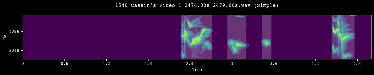
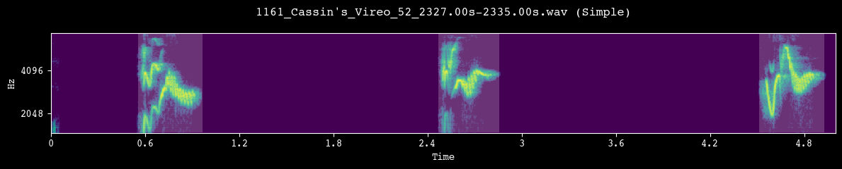
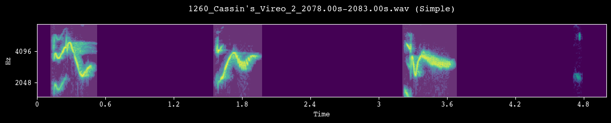
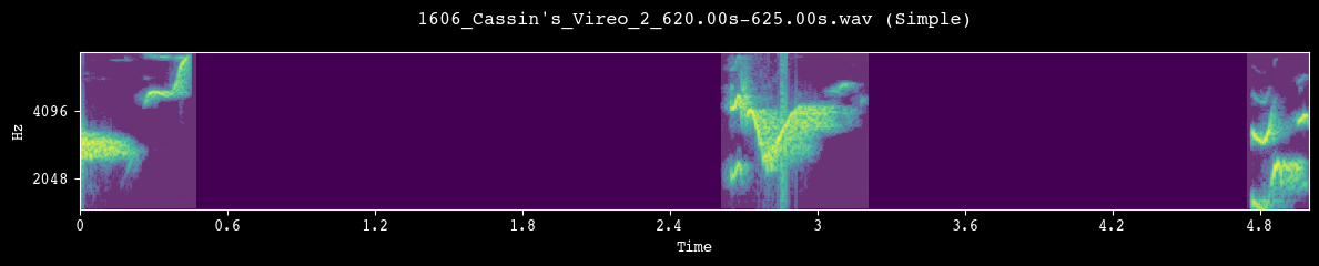
Before committing to a full segmentation run, we visually inspect a few random clips. Each call to demo_segmentation() selects a file from processed_dir, runs the chosen segmentation method, and plots the spectrogram with detected unit boundaries overlaid.

# preview the segmentation pipeline
analyzer.demo_segmentation(input_dir=processed_dir, simple=True)
analyzer.demo_segmentation(input_dir=processed_dir, simple=True)
analyzer.demo_segmentation(input_dir=processed_dir, simple=True)
analyzer.demo_segmentation(input_dir=processed_dir, simple=True)

--- Demoing segmentation for: 1540_Cassin's_Vireo_1_2474.00s-2479.00s.wav ---
   Segment: 0.00s - 5.00s

--- Demoing segmentation for: 1161_Cassin's_Vireo_52_2327.00s-2335.00s.wav ---
   Segment: 1.66s - 6.66s

--- Demoing segmentation for: 1260_Cassin's_Vireo_2_2078.00s-2083.00s.wav ---
   Segment: 0.00s - 5.00s

--- Demoing segmentation for: 1606_Cassin's_Vireo_2_620.00s-625.00s.wav ---
   Segment: 0.00s - 5.00s

After we are satisfied with the segmentation behavior, we apply it to the full dataset. segment_and_create_spectrograms() runs segmentation on every file in processed_dir, slices the corresponding spectrograms into fixed-size units, writes them to h5_path, and builds the unit_df metadata table used by the model.

# segment units and save spectrograms
unit_df = analyzer.segment_and_create_spectrograms(
    processed_dir=processed_dir, h5_path=h5_path, csv_path=csv_path, simple=True
)

--- Found 714 files to segment using simple (amplitude-based) method ---

Segmenting and saving spectrograms: 100%|██████████| 714/714 [00:08<00:00, 84.37it/s]

--- Data preparation complete. Created records for 2692 units ---
Spectrograms saved to /Volumes/Expansion/data/chatter/examples/cassins_vireo/spectrograms.h5
Unit metadata saved to /Volumes/Expansion/data/chatter/examples/cassins_vireo/spectrograms.csv

Run model

With segmented unit spectrograms in hand, we fit a convolutional variational autoencoder (VAE) that learns a low-dimensional representation (latent space) of Cassin’s vireo syllables.

The modeling workflow here has four main steps:

1. Train the autoencoder (train_ae):

   • Uses unit_df and h5_path to draw batches of unit spectrograms.

   • Optimizes a reconstruction + KL-divergence loss over multiple epochs.

   • Saves the best-performing model parameters and a loss history CSV to model_dir.

2. Reload the trained model (Trainer.from_trained):

   • Demonstrates how to restore a model from disk using just the config and model_dir.

   • This is the entry point you would typically use in downstream analysis notebooks.

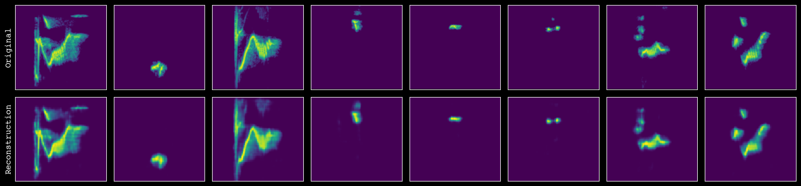
3. Inspect reconstructions (plot_reconstructions):

   • Plots original vs. reconstructed spectrograms for a subset of units.

   • Helps you visually assess whether the model is capturing relevant structure without overfitting.

4. Extract latent features (extract_and_save_features):

   • Runs all units through the encoder to obtain latent vectors and related diagnostics.

   • Writes a new CSV (output_csv_path) that augments unit_df with these model-derived features.

The remainder of the notebook shows how to work with this feature table to produce visualizations and summary statistics.

We now train the autoencoder on all segmented units. train_ae() reads batches of spectrograms from h5_path using the indices in unit_df, optimizes the VAE for a fixed number of epochs, and saves the trained model and loss history to model_dir.

# train ae
model.train_ae(unit_df=unit_df, h5_path=h5_path, model_dir=model_dir, subset=1)

--- Training on the full dataset of 2692 units ---

Starting training for 100 epochs using 4 DataLoader workers...

Training model: 100%|██████████| 100/100 [09:39<00:00,  5.79s/it, loss=1171.2967]

--- Training complete. Model saved to /Volumes/Expansion/data/chatter/examples/cassins_vireo/model/model.pth ---
Loss history saved to /Volumes/Expansion/data/chatter/examples/cassins_vireo/model/loss.csv

This cell shows how to reload a previously trained model. Trainer.from_trained() reconstructs the Trainer with weights and optimizer state from model_dir, which is the typical starting point for analysis notebooks that consume a trained model.

# load trained vae
model = chatter.Trainer.from_trained(config, model_dir)

Instantiating Trainer from pre-trained model at /Volumes/Expansion/data/chatter/examples/cassins_vireo/model...
Initializing convolutional variational autoencoder
Using device: mps
Successfully loaded pre-trained model from /Volumes/Expansion/data/chatter/examples/cassins_vireo/model/model.pth

Before trusting the model for feature extraction, we visually inspect its reconstructions. plot_reconstructions() shows side-by-side original and reconstructed spectrograms for a sample of units so you can check that key structure is being captured.

# assess the quality of reconstruction
model.plot_reconstructions(unit_df=unit_df, h5_path=h5_path)

Finally, we extract latent features for every unit and save them to disk. extract_and_save_features() runs the encoder on all spectrograms, attaches the resulting vectors and diagnostics to unit_df, and writes an augmented CSV to output_csv_path.

# export the latent features
output = model.extract_and_save_features(
    unit_df=unit_df,
    h5_path=h5_path,
    model_dir=model_dir,
    output_csv_path=output_csv_path,
)

--- Starting feature extraction ---
Successfully loaded pre-trained model from /Volumes/Expansion/data/chatter/examples/cassins_vireo/model/model.pth

Extracting features: 100%|██████████| 43/43 [00:06<00:00,  6.68it/s]

--- Pipeline complete. Exported data for 2692 units to /Volumes/Expansion/data/chatter/examples/cassins_vireo/output.csv ---

Postprocessing

At this point we have a table where each row is a segmented unit and columns include:

• Basic metadata (original file, onset, offset).

• Latent features from the trained VAE.

The FeatureProcessor class provides a convenient interface for turning these features into visualizations and higher-level acoustic measures:

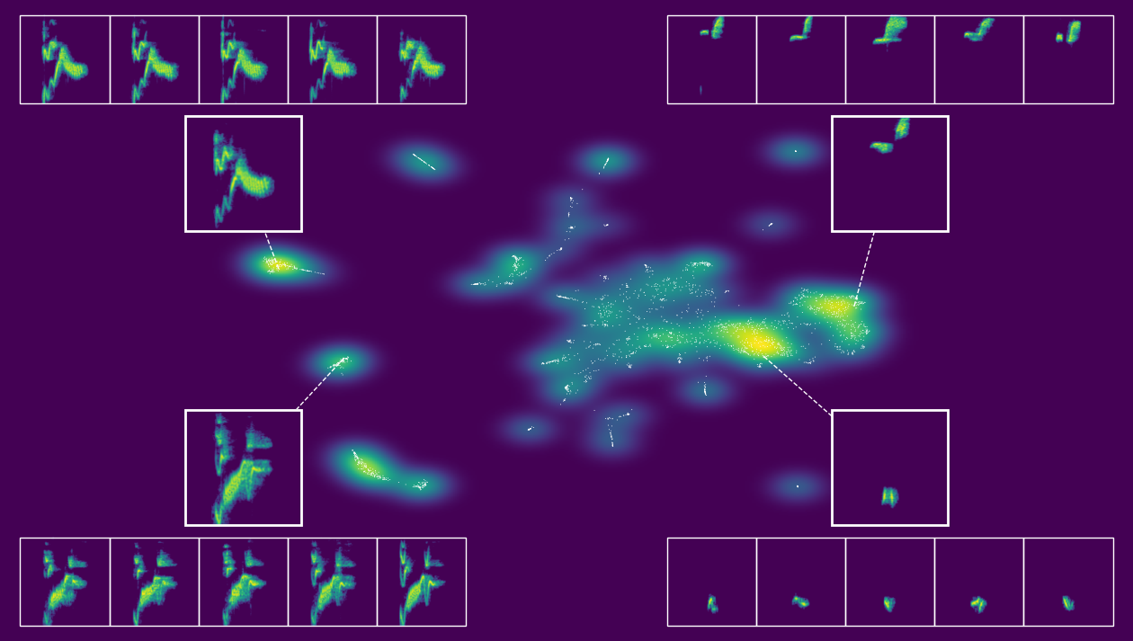
1. Load features into a processor (FeatureProcessor): wraps the DataFrame and config.

2. Dimensionality reduction and visualization:

   • run_pacmap() computes a 2D embedding of the latent space using PaCMAP, a more robust extension of UMAP.

   • static_embedding_plot() creates a publication-ready figure with points in latent space and overlaid spectrogram cutouts for representative units.

3. Sequence-level structure:

   • assign_sequence_ids() groups units into sequences based on temporal proximity (here using a 1-second gap threshold between units).

4. Standard acoustic measures:

   • compute_frequency_statistics() calculates summary statistics (e.g., frequency quantiles) that are commonly used in birdsong research.

5. Neighborhood and transition statistics:

   • compute_density_probability() estimates how densely populated each point is in latent space, by fitting a masked autoregressive flow with the denmarf package.

   • compute_cosine_distances() measures the path length between subsequent units within a sequence, using the cosine distance.

   • compute_sse_resid() fits a simple vector autoregression (VAR) model to sequences and uses residuals as a measure of transition likelihood.

6. Export results:

   • Finally, we write the enriched DataFrame back to output_csv_path, creating a single CSV that contains unit-level metadata, model-derived features, and a rich set of postprocessed measures.

You can treat this final CSV as the main output of the Chatter pipeline for downstream statistical analysis, visualization, or integration with behavioral and ecological data. Note that the reduced dimensions from PaCMAP are used only for visualization, and all other analyses are run on the original embeddings from the VAE.

We now wrap the feature CSV in a FeatureProcessor. This helper class keeps the DataFrame and config together and exposes convenience methods for dimensionality reduction, plotting, and calculating additional acoustic statistics.

# load in latent features
output = chatter.FeatureProcessor(analyzer.load_df(output_csv_path), config)

Attempting to load /Volumes/Expansion/data/chatter/examples/cassins_vireo/output.csv...
--- Successfully loaded /Volumes/Expansion/data/chatter/examples/cassins_vireo/output.csv ---

To make the high-dimensional latent features easier to explore, we first compute a 2D embedding. run_pacmap() applies the PaCMAP algorithm to the latent vectors and stores the resulting coordinates in the feature table.

# run pacmap to get two-dimensional embedding for visualization
output.run_pacmap()

--- Running PaCMAP dimensionality reduction ---
--- PaCMAP complete ---

<chatter.features.FeatureProcessor at 0x341957cb0>

Now we create a 2D visualization of the latent space. static_embedding_plot() uses the PaCMAP coordinates to produce a publication-ready figure with unit points, density shading, and overlaid spectrogram callouts for informative examples. By playing around with the seed we can modify which points are shown.

# create static plot
output.static_embedding_plot(
    h5_path=h5_path,
    seed=11,
    focal_quantile=0.5,
    point_size=0.5,
    point_alpha=1,
    margin=0.01,
    zoom_padding=0.42,
    num_neighbors=5,
)

--- Automatically selecting focal points from quadrants with seed 11 ---
--- Finding nearest neighbors ---
--- Creating the plot ---
--- Plotting density background (using fast 2d histogram) ---
--- Calculating callout positions and adding spectrograms ---
--- Displaying plot ---

<chatter.features.FeatureProcessor at 0x341957cb0>

We can also create an interactive version of this. The actual output of export_interactive_embedding() is an HTML file, but the example below is a screen capture of it.

# create interactive plot
output.interactive_embedding_plot(
    h5_path=h5_path, output_html_path=output_html_path, point_alpha=1, point_size=1
)

--- Encoding spectrogram thumbnails for HTML export ---

Thumbnails: 100%|██████████| 2692/2692 [00:02<00:00, 1332.59it/s]

--- Interactive HTML embedding saved to /Volumes/Expansion/data/chatter/examples/cassins_vireo/cassins_vireo_embedding.html ---

<chatter.features.FeatureProcessor at 0x385467cb0>

After visualizing the embedding, we group units into temporal sequences. assign_sequence_ids() walks through units ordered by time and starts a new seq_id whenever the gap between adjacent units exceeds the specified cutoff (here 1 second).

# assign sequence ids based on the 1-second cutoff
output.assign_sequence_ids()

--- Assigning seq_id using seq_bound = 1.0 seconds ---
--- seq_id assignment complete; total sequences: 1690 ---

<chatter.features.FeatureProcessor at 0x341957cb0>

Here we use compute_frequency_statistics() to compute standard acoustic measures familiar from birdsong research: minimum, mean, and maximum frequency.

# calculate standard acoustic measures used in birdsong research
output.compute_frequency_statistics(h5_path=h5_path)

--- Computing frequency statistics from spectrograms ---

Analyzing spectrograms: 100%|██████████| 2692/2692 [00:01<00:00, 1483.02it/s]

--- Frequency statistics computation complete ---

<chatter.features.FeatureProcessor at 0x341957cb0>

We also estimate how densely populated each point is in the latent space. compute_density_probability() assigns a density-based score to each unit, which can be useful for identifying rare or typical syllables.

# compute density probability of each unit
output.compute_density_probability()

--- Computing density probability estimates using denmarf ---
    Using 32-dimensional latent feature space.
    Fitting MAF model on 2692 samples (device: mps)...

current average log likelihood: nan: 100%|██████████| 1000/1000 [07:31<00:00,  2.21it/s]

best average log likelihood: -41.249
    Scoring samples...
--- Density estimation complete. Added 'density_log_prob' to DataFrame ---

<chatter.features.FeatureProcessor at 0x341957cb0>

Next we quantify the path length between subsequent units in sequences. compute_cosine_distances() computes cosine distances between successive latent vectors, which can be interpreted as a measure of acoustic change rate over time.

# compute cosine distances between subsequent units in sequences
output.compute_cosine_distances()

--- Computing cosine distances between subsequent syllables (within seq_id) ---
--- Cosine distance calculation complete (within seq_id only) ---

<chatter.features.FeatureProcessor at 0x341957cb0>

Here we estimate how surprising each unit-to-unit transition is. compute_sse_resid() fits a simple vector autoregression (VAR) model to sequences in latent space and uses the summed squared residuals as a measure of transition likelihood (larger values indicate less expected transitions given recent context).

# compute the likelihood of each transition between units
output.compute_sse_resid()

--- Running global VAR model (OLS) with lag size p = 3 ---
--- Global VAR model (OLS) complete; sse_resid computed for all sequences ---

<chatter.features.FeatureProcessor at 0x341957cb0>

Before finishing, we save the enriched feature table back to disk. This CSV combines unit-level metadata, VAE-derived features, sequence IDs, and all postprocessed measures so it can be used in downstream analyses or other software. Note that the first unit of each sequence is given NaN for cosine_dist and sse_resid, since those values are relative to the first unit in each sequence.

# preview the final data frame
output.df

	source_file	unit_index	onset	offset	max_unit_length_s	h5_index	ae_feat_0	ae_feat_1	ae_feat_2	ae_feat_3	...	pacmap_x	pacmap_y	seq_id	min_freq	mean_freq	max_freq	time_bin_ms	density_log_prob	cosine_dist	sse_resid
0	hedley_2016/Wav Files 1/1113_Cassin's_Vireo_1_...	0	0.031927	0.374422	0.8	1971	1.410389	-2.699534	1.295568	0.646331	...	8.095862	-2.044903	1	1500.000000	2375.142101	7129.297213	6.25	-42.518436	NaN	NaN
1	hedley_2016/Wav Files 1/1113_Cassin's_Vireo_1_...	1	0.641451	0.873651	0.8	1972	-0.976862	0.353828	-1.931226	1.852069	...	6.673967	-2.631289	1	2138.929378	2505.763628	2936.216478	6.25	-26.115707	1.052800	62.332695
2	hedley_2016/Wav Files 1/1113_Cassin's_Vireo_1_...	2	1.439637	1.843084	0.8	1973	3.946225	-3.297062	-0.347933	0.368604	...	-13.315022	-14.799085	1	1500.000000	3724.592170	6776.916971	6.25	-37.763107	1.167537	149.182406
3	hedley_2016/Wav Files 1/1113_Cassin's_Vireo_1_...	3	3.604898	4.028662	0.8	1974	3.209291	-1.472756	0.012070	-0.722493	...	-13.210196	-14.569655	2	1500.000000	3798.581942	6524.135804	6.25	-34.966949	NaN	NaN
4	hedley_2016/Wav Files 1/1113_Cassin's_Vireo_1_...	4	4.040272	4.159274	0.8	1975	0.337892	2.038742	1.111712	0.800808	...	10.202535	2.893551	2	4575.301882	4725.160134	4936.733992	6.25	-10.372253	1.059631	43.464143
...	...	...	...	...	...	...	...	...	...	...	...	...	...	...	...	...	...	...	...	...	...
2687	hedley_2016/Wav Files 3/1841_Cassin's_Vireo_1_...	0	0.000000	0.121905	0.8	778	-0.982202	3.746105	1.258669	0.656011	...	9.680232	2.545646	1689	4082.121425	4608.508021	5326.771592	6.25	-12.080605	NaN	NaN
2688	hedley_2016/Wav Files 3/1841_Cassin's_Vireo_1_...	1	1.233560	1.613787	0.8	779	0.207171	-1.890158	0.973335	5.958722	...	-1.043776	-3.734445	1690	1500.000000	3639.036725	7312.345246	6.25	-46.577782	NaN	NaN
2689	hedley_2016/Wav Files 3/1841_Cassin's_Vireo_1_...	2	1.950476	2.089796	0.8	780	1.633583	2.349890	0.771327	1.764572	...	10.795265	2.308394	1690	4460.767812	4973.235868	5394.703807	6.25	-17.789322	1.130541	100.897193
2690	hedley_2016/Wav Files 3/1841_Cassin's_Vireo_1_...	3	2.385850	2.528073	0.8	781	-0.562219	0.969748	-0.693975	2.147093	...	6.591626	-2.115031	1690	1791.207173	2374.763711	3128.292871	6.25	-26.665470	0.849881	201.754410
2691	hedley_2016/Wav Files 3/1841_Cassin's_Vireo_1_...	4	3.111474	3.538141	0.8	782	-1.515847	-2.088365	1.086043	-0.465359	...	-0.342227	-11.511266	1690	1519.137359	3519.481183	6360.844448	6.25	-39.351994	0.847840	74.121701

2692 rows × 48 columns

# save the final data frame with all of these measures to a CSV file
output.df.to_csv(output_csv_path, index=False)